
Overview
Akhilandeshwari Krishnan is a high school freshman newly working with DoseNet at UC Berkeley. Her first project in Summer 2022 focused on spectral data analysis and obtaining net counts from a peak. Akhila put together a report of the multiple procedures used and the resulting counts of significant peaks in data from the rooftop Cesium Iodide sensor.
Introduction
This summer, my project was to build a tool that extracted the net counts of radiation from a given peak in a spectrum. After cleaning spectral data, two functions were created for obtaining the net counts of a peak, with one function using integration and the other utilizing background subtraction with a choice of two procedures. Using several methods of extracting net counts allowed comparison and contrast between different procedures, and helped determine the limitations of each. The net counts of the peak were then graphed into plots. This tool was used in analysis of data from DoseNet’s rooftop Cesium Iodide sensor.
Procedures
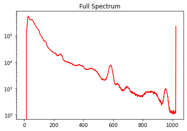
Data was taken from the rooftop sensor on Etcheverry Hall with a focus on calculating the net counts of radiation from the Potassium-40 peak in particular. Input data representing KeV and counts per minute were read into a Pandas dataframe from a csv file. Data often includes missing or NaN values that have to be cleaned, so these non-numerical values were forward-filled to avoid miscalculations. This complete spectrum was then plotted as a reference dataset for selecting peaks. Below is the spectrum of the rooftop Cesium Iodide sensor on Etcheverry Hall. As shown in the figure, there are multiple significant peaks visible.
Figure 1. Etcheverry Roof Cesium Iodide full spectrum plot
Net Counts (tail-trained background): 25676.10312889503
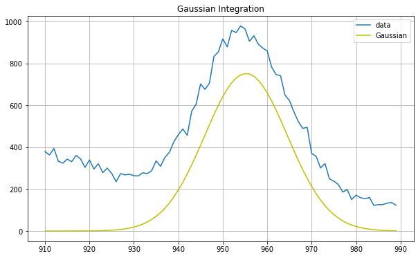
Integration
The first method to isolate the net counts of a peak used integration to sum all the counts of a peak. The function accepts an array of x and y values each, the peak’s left bound and right bound, and Gaussian curve estimates as arguments from the user. A Gaussian fit is generated for the specified peak. Then the Gaussian is integrated, essentially summing all radiation counts under the curve. Figure 2 shows the Thallium-208 peak’s results using integration.
Figure 2. Thallium-208 peak net counts (integration)
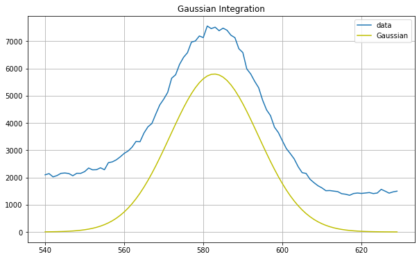
Net Counts: 17504.21875021408
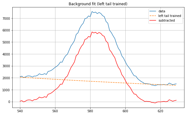
Background Subtraction (Left-tail Trained)
Another approach was to determine and subtract the background radiation from the peak. Background counts come from the radiation bouncing off every surface in the environment, usually in miniscule doses but varying depending on location. The function accepts an array of x and y values as input data, the peak’s left bound and right bound, and estimate values for an exponential curve as arguments from the user. Optionally, tail length around the peak can be specified, as well as a starting offset in case of noise early in the data. An exponential fit is then generated, trained on the left tail, and used to interpolate between the peak’s bounds. The model is not right- or two-tail trained because of sensor settling noise; often sensors experience momentary ‘bouncing’ to settle after detecting a significant peak and such noise can cause miscalculations. After interpolation, the background values are subtracted from the peak’s values, resulting in the net counts. The original peak data, background fit, and net-count peak are all plotted on a graph. Figure 3 shows results from another significant peak, using left-tail training for background subtraction.
Figure 3. Significant peak net counts (tail-trained background subtraction)
Net Counts (tail-trained background): 25676.10312889503
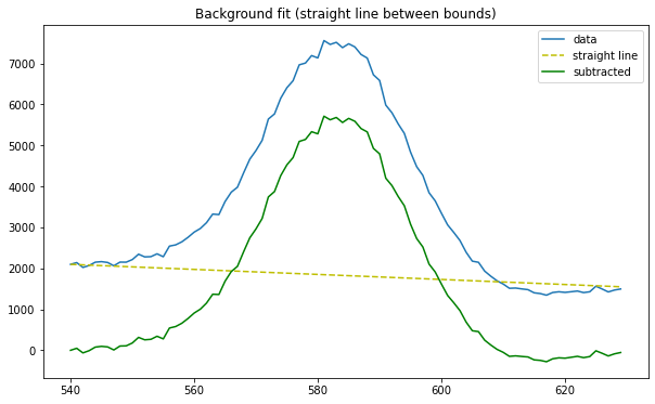
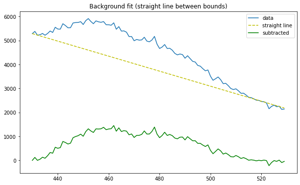
Background Subtraction (Linear Estimator)
An option in the background subtraction function was built in case of particularly noisy or unusable data, where training a model on the left tail would produce inaccurate results. This procedure simply generates a straight line between peak bounds as a background fit. The linear estimate’s values are subtracted from the peak’s values, resulting in the net counts. The original peak data, linear estimate, and net-count peak are all plotted on a graph. Figure 4 shows results from a smaller peak, using linear-estimate background subtraction and resulting in 66984.17000000009 net counts.
Figure 4. Smaller peak net counts (liner-estimate background subtraction)
Net Counts (linear-estimate background): 66984.17000000009
Comparison of Methods
Integration using a Gaussian fit is excellent when given good starting estimates. Background subtraction using left-tail training works well for peaks with level tails, but requires adjusting the training tail length when noisy tails are present. Background subtraction using linear estimation is a viable option for peaks with level tails. However, the line cuts through peaks with uneven tails. Using multiple procedures to calculate net counts allows the user to try them all and determine the best option for specific conditions.
Conclusion
Net counts from the Potassium-40 peak were calculated using all three methods. The figures below illustrate each. Integration resulted in 162684.86434594737 counts and left-tail background subtraction resulted in 167310.97734118442 counts. These values are quite close to each other, however the linear-estimate background option for this particular peak is (even visually on the plot) a somewhat inaccurate method choice at 155638.5722222222 counts.
Next steps could involve using Plotly instead of Matplotlib to provide interactive graphs instead of static representations. One observation is that the left-tail trained background model is extremely sensitive. Further work would try to improve this oversensitivity and achieve greater accuracy.
Figure 5. Potassium-40 peak net counts (tail-trained background subtraction)
Net Counts (tail-trained background): 167310.97734118442
Figure 6. Potassium-40 peak net counts (liner-estimate background subtraction)
Net counts (linear-estimate background): 155638.5722222222
Figure 7. Potassium-40 peak net counts (integration)
Net Counts: 162684.86434594737
All graphs were generated using the Matplotlib library in Python. NumPy and SciPy libraries in Python were used for data processing.