DoseNet Summer 2024: Esther Luvishis’ Report

Research on Radiation Dose around Medical Procedures and Small Aircraft

Esther Luvishis

Introduction

Radiation is used in a variety of medical procedures, so it’s not uncommon to see signs that warn of Radioactive Materials or that Caution for Radiation. This research was conducted in order to test the dose that one would get in a hospital, and to investigate radiation next to a portable PET scanner. Data for this was collected on a Cesium-Iodide (CsI) crystal detector. The findings concluded that the dose someone passing by, or even standing near it, receives is NOT significant, and is greatly below government regulations.

Portable PET Scan

PET stands for Positron-electron tomography. These scans use radioactive tracers, to see where gamma rays are given off. In the city where I live, there are several portable PET scanners. The only radioactive part of the procedure should be the patient injucted with radiotracers. In order to get the information needed for dose, I took 3, 10 minute measurements at 5 step intervals(using my feet as measurement) stepping away from the PET scanner. The closest trial had a mean of 3266.11 CPS. The farthest trial had a mean of 344.09 CPS when peaks are taken away. (Peak count rates were detected when a person walked by, their body containing the various sources I explore in this paper) Using that, we can conclude that I was originally 4.8 feet away from the source. If we assume that 40 CPS is normal background, then it would take approximately 43 feet to get back to background. I’d also like to mention that in some trials there were inconsistencies in radiation detection, sometimes the background level was higher, and sometimes a person with the source wouldn’t be detected as a spike.

Calculations for Range from PET Scanner

To determine the effective range from the PET scanner to background radiation levels, we start with:

Inline equation:

\( R_1 = \frac{3266.11}{344.09} \)

The original distance from the source (\(d_1\)) was:

\( d_1 = 4.8 \, \text{feet} \)

Assuming normal background radiation is approximately \( 40 \, \text{CPS} \), the range (\( d_2 \)) required to reach background level can be calculated as:

\[ d_2 = d_1 \times \sqrt{\frac{R_1}{40}} \]

Substituting the values:

\[ d_2 = 4.8 \times \sqrt{\frac{3266.11}{40}} \approx 43 \, \text{feet} \]

Thus, it takes approximately 43 feet to get back to the background radiation level.

From there we can also figure out what radioactive source specifically was being used, that also might there be on a more consistent basis, because the data showed a consistent level of counts besides people walking past. We can do this by figuring out the half life, from a fitted line of Ae-λt+b.(this is the equation for half life decay) This gave us a slope of the exponential of 0.000489. This is manipulated to give us a half life of 1417.47 seconds, or 23.62 minutes. This is extremely close to the true half-life of carbon 11 --20 minutes. They often use carbon 11 for PET scans.

Calculations for Half-Life of the Radioactive Source

To determine the half-life (\( t_{1/2} \)) of the radioactive material, we use the exponential decay model:

\[ A(t) = A_0 e^{-\lambda t} + b \]

Where:

  • \( A(t) \) is the activity at time \( t \).
  • \( \lambda \) is the decay constant.
  • \( A_0 \) is the initial activity.
  • \( b \) is the offset constant.

We have found the decay constant (\( \lambda \)) to be:

\[ \lambda = 0.000489 \]

The half-life formula is given by:

\[ t_{1/2} = \frac{\ln(2)}{\lambda} \]

Substituting the value of \( \lambda \):

\[ t_{1/2} = \frac{\ln(2)}{0.000489} \]

Calculating this:

\[ t_{1/2} \approx 1417.47 \, \text{seconds} \approx 23.62 \, \text{minutes} \]

This calculated value of the half-life is very close to the actual half-life of Carbon-11, which is approximately 20 minutes. Carbon-11 is often used in PET scans.

Portable PET Scanner

Trial nearest PET scanner

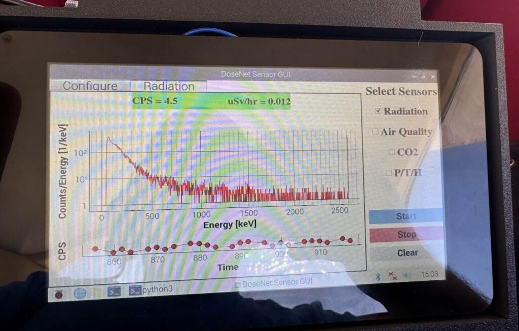
Example of what CsI detector looks like right next to PET scanner(notice peak around 511 keV. (Energy of tracer for PET scan)

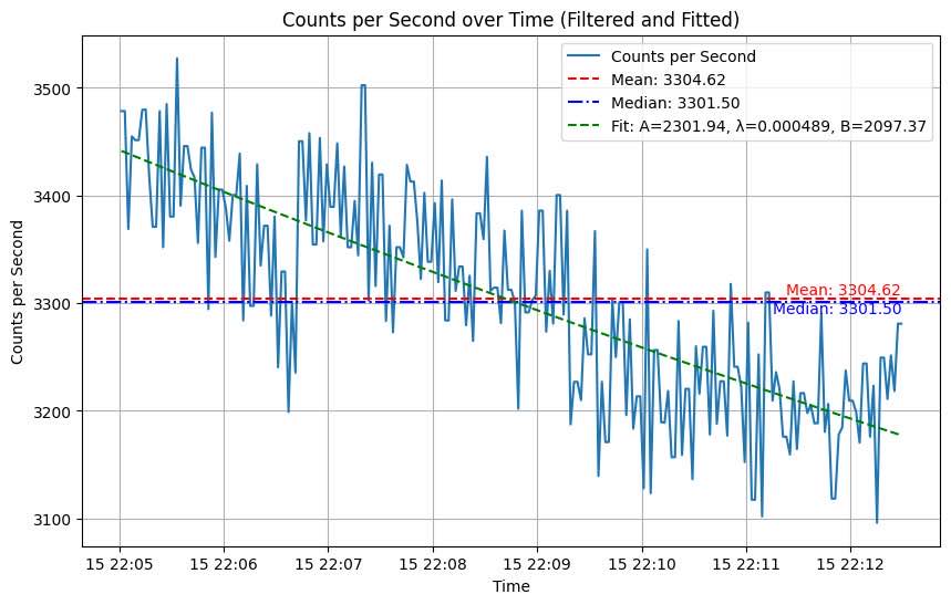
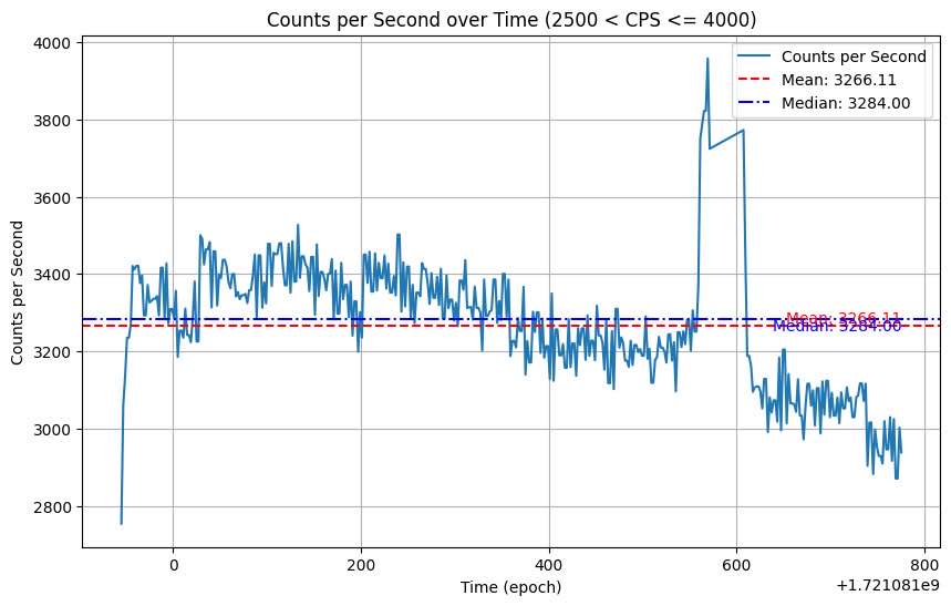
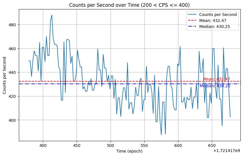
Finding half life decay with filtered data

Radiation Area in Hospital

The data for this was collected in a similar way. I stood by a door labeled Radioactive Material Storage, then took 5 steps back, and then another 5 steps. Using the same methods as above, we find that I was standing around 5.27 feet away from the source, and that’s about 17.33 feet away from background levels.

We begin by determining the ratio between the measured radiation levels (\( R_1 \)) and the background level (\( R_2 \)). Given the data: \[ R_1 = 432.47 \, \text{CPS}, \quad R_2 = 40 \, \text{CPS} \] The initial distance from the source (\( d_1 \)) was: \[ d_1 = 5.27 \, \text{feet} \] We want to determine the distance (\( d_2 \)) at which the radiation reaches background levels. This is given by the relationship: \[ d_2 = d_1 \times \sqrt{\frac{R_1}{R_2}} \] Substituting the values: \[ d_2 = 5.27 \, \text{feet} \times \sqrt{\frac{432.47 \, \text{CPS}}{40 \, \text{CPS}}} \] The units of CPS (counts per second) cancel out: \[ d_2 = 5.27 \times \sqrt{\frac{432.47}{40}} \, \text{feet} \] Simplifying the calculation: \[ d_2 = 17.33 \, \text{feet} \] Thus, the estimated distance required to reach background radiation levels is approximately \( 17.33 \, \text{feet} \).

Radiation Area in Hospital

From here, in order to get the true dose, we need to calculate the efficiency of the CsI device. This is done by using a known source, and finding the average CPS, and the activity we know about that source. This was especially important to do, to see the efficiency of the device at low energy levels, because that’s what the CsI device was showing. We found an efficiency of 0.0006904. This is used to find the activity, 626399.38 decays/second. Then from there, we can find the actual dose using the mass of an average male: 70 kg, and average energy of trial.

To determine the true dose, we start by calculating the efficiency of the CsI device. We use a known radioactive source, measure the average counts per second (CPS), and compare this to the known activity: \[ \text{Efficiency} = \frac{\text{CPS}}{\text{Activity}} \] Given: \[ \text{Activity} = 381816 \, \text{decays/second}, \quad \text{CPS} = 249.80 \] The efficiency (\( \epsilon \)) is: \[ \epsilon = \frac{249.80}{381816} = 0.000654 \] Using this efficiency, we calculate the activity of the source measured in the trial: \[ \text{Activity} = \frac{432.47 \, \text{CPS}}{0.000654} = 661024.68 \, \text{decays/second} \] Next, we calculate the dose using the following formula: \[ \text{Dose} = \frac{\text{Energy} \times \text{Activity}}{\text{Mass}} \] Where: - \( \text{Energy} \) is in joules. - \( \text{Activity} = 661024.68 \, \text{decays/second} \) - \( \text{Mass} = 70 \, \text{kg} \) Given: \[ \text{Energy} = 112.43 \, \text{keV} = 112430 \, \text{eV} \] Converting energy to joules (\( 1 \, \text{eV} = 1.60218 \times 10^{-19} \, \text{J} \)): \[ \text{Energy} = 112430 \times 1.60218 \times 10^{-19} \, \text{J} = 1.80088 \times 10^{-14} \, \text{J} \] Substituting into the dose formula: \[ \text{Dose} = \frac{1.80088 \times 10^{-14} \times 661024.68}{70} \] \[ \text{Dose} = 1.70103 \times 10^{-10} \, \text{Grays/second} \] Considering a 75\% absorption rate (which is an estimate to account for partial absorption of gamma rays): \[ \text{Effective Dose} = 0.75 \times 1.70103 \times 10^{-10} = 1.27578 \times 10^{-10} \, \text{Grays/second} \] To convert to microsieverts per hour: \[ \text{Dose Rate} = 1.27578 \times 10^{-10} \times 3.6 \times 10^3 = 0.459 \, \mu\text{Sv/hour} \] The federal limit in hospitals is: \[ \text{Limit} = 0.02 \, \text{mSv/hour} = 20 \, \mu\text{Sv/hour} \] The levels we found are well below the federal limit, making the radiation exposure completely safe.

Radiation Area in Hospital

In order to get the average energy of the trial, we had to convert channels to energy levels. This is done by finding background energy, and getting a K-40 peak: 1461 keV, at the index 577. Then additionally finding the peaks for energy levels 2614 keV, and 609 keV, we are able to get a quadratic calibration curve. The Quadratic Coefficients are: [8.19677055e-04 1.88560370e+00 1.00112405e+02] This calibration is done because the device is not as well calibrated to be used in low-energy situations, like the X-rays that we were seeing. Then, we used this to find the accurate average energy levels. From this we have to take into account a 75% absorption rate, and we get 1.2073×10⁻¹⁰ grays/s. This is converted to 0.434628 microsieverts/hour. The federal limit in hospitals is not to have more than 0.02 millisieverts/hour. Converting that to microsieverts gets us 20 microsieverts, so the levels we were finding are well below standard, and so are completely safe!

Spectrum-notice a lot of low energy peaks


First trial next to Storage
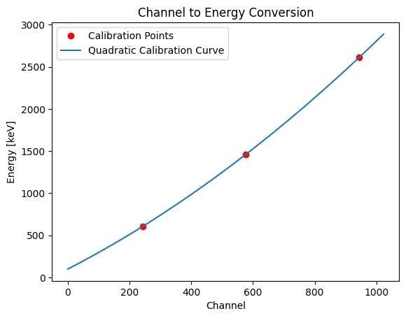
Calibration Curve

Part two

Introduction

Historically planes are known to have higher levels of radiation, going so far as to have regulations for people whose jobs include flying extremely often. This is because the higher altitude you have, the more exposure to cosmic rays you are getting, especially the closer to the poles you are. I got the opportunity to fly in a Cessna over the summer, so I brought the CsI detector with me in the air. The main discoveries we found were that the CsI detector cannot detect the most common cosmic rays. This is shown in the fact that we got less than background levels while at an altitude of around 5500 feet, seeing the drop off of the gamma rays reflected from the ground. From there we were able to show the actual correlations that could be picked up by the CsI.

Low cps levels, while at high altitude

Method

I found online data that tracked our planes altitude, vs time. This had to be calibrated to our time on the device. Unfortunately, the device's time wasn’t accurate because it hadn’t connected to the internet before. This meant that I had to first change all the times to the accurate epoch time, and then convert all the times from the website into the same format. The other problem was that their timing in between data points wasn’t the same, so a pandas data frame resample was used to fix that. Lastly, there were some problems with delays that contributed to uncertainty with the take off and landing times correlated to the graph in terms of background radiation, so the data was shifted to account for that. Doing all this, gives us a correlation of around -0.85 between Radiation Counts and Altitude, showing how only the altitude was contributing to radiation differences!


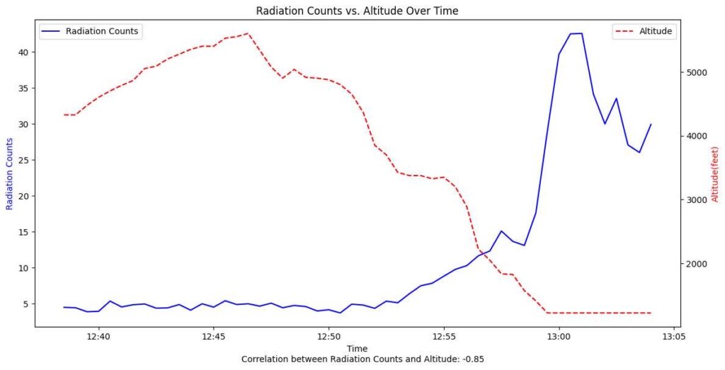
Correlation graph between Radiation Counts, and Altitude over Time

Scatterplot

Next, we made a scatterplot to look at the specific data points. We focused on the region below 4000 ft, but above the ground because we wouldn’t expect fluctuations on the groups to be related to change in altitude, and above a certain altitude. (It flattens off around 4000 ft) For that specific section, there was a very strong correlation of -0.95. The p-value was also minuscule enough that it showed up at 0.0000, meaning that there is a 0% chance that such a correlation was due to random chance, proving a statistically significant correlation.


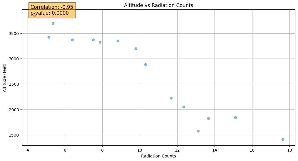
Scatterplot with Altitude vs Radiation Counts


Acknowledgments

HUGE thank you to Dr Hanks, who helped me with everything, and Gilder who helped me find the efficiency data. And to Dani a huge thanks for helping me put together this article! 🙂


Me flying 🙂

Posted in Education, Internship.